Phasor activation functions
MVN activation function
This code explains the logic of mvn activation function for an easy understanding.
For further information refer to the original papers of Naum Aizenberg:
According to these works: A multi-valued neuron (MVN) is a neural element with n inputs and one output lying on the unit circle, and with complex-valued weights.
[ ]:
# We first import everything
import matplotlib.pyplot as plt
from cvnn.activations import mvn_activation, georgiou_cdbp
import tensorflow as tf
import numpy as np
For a start we will create complex valued points to use as an example.
[ ]:
x = tf.constant([-2, 1.0, 0.0, 1.0, -3], dtype=tf.float32)
y = tf.constant([-2.5, -1.5, 0.0, 1.0, 2], dtype=tf.float32)
z = tf.complex(x, y)
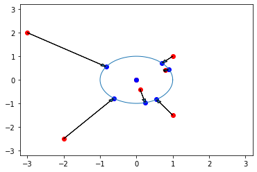
MVN function divides the phase into k sections and cast the input phase to the closest of those k values while also fizing the amplitude to 1.
The equation would be
with \(a\) so that
[ ]:
k = 3
result = mvn_activation(z, k=k)
# cnums = np.arange(5) + 1j * np.arange(6, 11)]
ax = plt.axes()
ax.scatter(tf.math.real(z), tf.math.imag(z), color='red')
ax.scatter(tf.math.real(result), tf.math.imag(result), color='blue')

# Plot arrows of the mapping road
for x, y, dx, dy in zip(tf.math.real(z), tf.math.imag(z),
                        tf.math.real(result) - tf.math.real(z),
                        tf.math.imag(result) - tf.math.imag(z)):
    ax.arrow(x, y, dx, dy, length_includes_head=True, head_width=0.1)
# PLot unit circle
t = np.linspace(0, np.pi * 2, 100)
ax.plot(np.cos(t), np.sin(t), linewidth=1)

yabs_max = abs(max(ax.get_ylim(), key=abs))
xabs_max = abs(max(ax.get_xlim(), key=abs))
axis_max = max(yabs_max, xabs_max)

# Divide map on the different zones
ax.pie(np.ones(k) / k, radius=4, wedgeprops={'alpha': 0.3})

ax.set_ylim(ymin=-axis_max, ymax=axis_max)
ax.set_xlim(xmin=-axis_max, xmax=axis_max)
plt.show()
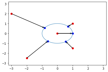
Continous values
If k is not given, it will use \(k \to \infty\) making it an equivalence of just mapping the input to the unitary circle (keeps the phase but changes the amplitude to 1). This is mathematically
For \(z \neq 0\) this is also
[ ]:
result = mvn_activation(z)

ax = plt.axes()
ax.scatter(tf.math.real(z), tf.math.imag(z), color='red')
ax.scatter(tf.math.real(result), tf.math.imag(result), color='blue')
for x, y, dx, dy in zip(tf.math.real(z), tf.math.imag(z),
                        tf.math.real(result) - tf.math.real(z),
                        tf.math.imag(result) - tf.math.imag(z)):
    ax.arrow(x, y, dx, dy, length_includes_head=True, head_width=0.1)
t = np.linspace(0,np.pi*2,100)
ax.plot(np.cos(t), np.sin(t), linewidth=1)

yabs_max = abs(max(ax.get_ylim(), key=abs))
xabs_max = abs(max(ax.get_xlim(), key=abs))
axis_max = max(yabs_max, xabs_max)

ax.set_ylim(ymin=-axis_max, ymax=axis_max)
ax.set_xlim(xmin=-axis_max, xmax=axis_max)
(-3.2, 3.2)
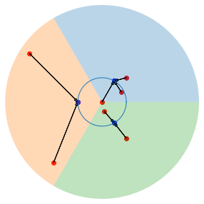
Georgiou CDBP
Activation function proposed by G. M. Georgioy and C. Koutsougeras
There are a few differences with MVN:
- You can choose the circle radius with the
rparameter. - Zero stays at zero.
[ ]:
x = tf.constant([-2, 1.0, 0.0, 1.0, -3, 0.8, 0.1], dtype=tf.float32)
y = tf.constant([-2.5, -1.5, 0.0, 1.0, 2, 0.4, -0.4], dtype=tf.float32)
z = tf.complex(x, y)
result = georgiou_cdbp(z)

ax = plt.axes()
ax.scatter(tf.math.real(z), tf.math.imag(z), color='red')
ax.scatter(tf.math.real(result), tf.math.imag(result), color='blue')
for x, y, dx, dy in zip(tf.math.real(z), tf.math.imag(z),
                        tf.math.real(result) - tf.math.real(z),
                        tf.math.imag(result) - tf.math.imag(z)):
    ax.arrow(x, y, dx, dy, length_includes_head=True, head_width=0.1)
t = np.linspace(0, np.pi * 2, 100)
ax.plot(np.cos(t), np.sin(t), linewidth=1)

yabs_max = abs(max(ax.get_ylim(), key=abs))
xabs_max = abs(max(ax.get_xlim(), key=abs))
axis_max = max(yabs_max, xabs_max)

ax.set_ylim(ymin=-axis_max, ymax=axis_max)
ax.set_xlim(xmin=-axis_max, xmax=axis_max)
plt.show()